Pythonの数値計算用モジュールの一つである Theano について、基本的な使い方を整理する。余裕があれば、最終的には 公式チュートリアル の和訳版とする。
事前準備
以下の3つは常にimportしておく。
import numpy as np
from theano import *
import theano.tensor as T
tensor サブモジュールは頻繁に使うので、扱いやすい名前 (ここではT) でimportしておく。
NumPyのおさらい
機械学習において、Theano と併せて使うことが多い NumPy モジュールについて、基本的な使い方 (主に行列演算の方法) を整理する。
そのうちまとめる
基本的な使い方
- シンボル (変数) の宣言
- 数式の定義
- 関数の生成
- Tips
- byte: bscalar, bvector, bmatrix, brow, bcol, btensor3, btensor4
- 16-bit integers: wscalar, wvector, wmatrix, wrow, wcol, wtensor3, wtensor4
- 32-bit integers: iscalar, ivector, imatrix, irow, icol, itensor3, itensor4
- 64-bit integers: lscalar, lvector, lmatrix, lrow, lcol, ltensor3, ltensor4
- float: fscalar, fvector, fmatrix, frow, fcol, ftensor3, ftensor4
- double: dscalar, dvector, dmatrix, drow, dcol, dtensor3, dtensor4
- complex: cscalar, cvector, cmatrix, crow, ccol, ctensor3, ctensor4
数値計算で変数として扱う記号をシンボルとして宣言する。
x = T.dscalar('x')
y = T.dscalar('y')
ここでは、倍精度浮動小数点数 (d, double) のスカラー (scalar) を表すシンボル x と y を宣言している。dscalar というクラスはなく、 x や y はあくまで TensorVariable クラスのインスタンスである。各インスタンスのtypeという変数に、変数の型を示す情報が収納される。
type(x)
x.type
T.dscalar
x.type is T.dscalar
<class 'theano.tensor.basic.TensorVariable'>
TensorType(float64, scalar)
TensorType(float64, scalar)
True
また、括弧の中の文字列はシンボルの名前を指定するもので、必須ではないが、名前を与えておくとエラーメッセージ上に表示されるためデバッグしやすくなる。シンボルの宣言についての詳細は、4. Tips で解説する。
1.で宣言したシンボルを組み合わせて、計算したい数式を定義する。
z = x + y
xやyは値を持たないシンボルなので、zにも具体的な値は入らず、‘x + y’ を意味するシンボルになる。theano.pp を用いることで、数式の中身を確認することができる。
print pp(z)
(x + y)
2.で定義した数式を実際に計算するための関数を生成する。関数は、 theano.function を用いて生成する。第1引数としてシンボルのリスト、第2引数として計算したい数式を与える。それぞれ、inputs・outputsというキーワード引数としても指定可能。
f = function([x, y], z)
# f = function(inputs=[x, y], outputs=z)
作成した関数に具体的な値を引数として与えて実行すると、数式の計算結果が返される。引数はNumPy配列 (numpy.array) として解釈され、戻り値もNumPy配列となる。
f(2, 3)
f(16.3, 12.1)
array(5.0)
array(28.4)
theano.function を呼び出した際に、対象の数式を実現するC言語の計算プログラムがコンパイルされる。そのため、この関数の実行には少し時間がかかる。1つの関数で複数の計算結果を出力したい場合は、outputsを数式シンボルのリストにすることもできる。この場合は、inputsに与える変数シンボルのリストが全ての数式をカバーしている必要がある。
y2 = T.dscalar('y2')
z2 = x + y2
f2 = function([x, y, y2], [z, z2])
f2(3, 5, 9)
[array(8.0), array(12.0)]
1.のシンボル宣言の際に、変数の型を適切に指定することで、スカラー演算のみならず、ベクトル演算や行列演算も計算できる。変数の型には、テンソルの階数(スカラー・ベクトル・行列などの次元的な概念)と数値の型があり、これらを組み合わせることによって指定する。例えば、dmatrix は、倍精度浮動小数点数 (d, double) の行列 (matrix) を意味する。
x = T.dmatrix('x')
y = T.dmatrix('y')
z = x + y
f = function([x, y], z)
f([[1, 2], [3, 4]], [[10, 20], [30, 40]])
array([[ 11.,  22.],
       [ 33.,  44.]])
指定できる変数の型は、以下の通り (公式チュートリアルより引用)。詳細はこちらも参照。
微分の計算
theano.tensor.grad を用いて微分を計算することができる。第1引数として微分の対象となる数式、第2引数として微分を取るシンボルを与える。それぞれ、 cost・wrt (with respect to ?) というキーワード引数としても指定可能。実際に数値を求めるためには、通常の数式と同じように関数を生成する必要がある。
x = T.dscalar('x')
y = x ** 2
gy = T.grad(y, x)
f = function([x], gy)
f(4)
f(94.2)
array(8.0)
array(188.4)
theano.pp を用いることで、微分式の中身を確認することができる。また、 theano.function.maker.fgraph.outputs[0] に対して theano.pp を用いることで、最適化された微分式を確認することができる。
pp(gy)
pp(f.maker.fgraph.outputs[0])
'((fill((x ** TensorConstant{2}), TensorConstant{1.0}) * TensorConstant{2}) * (x ** (TensorConstant{2} - TensorConstant{1})))'
'(TensorConstant{2.0} * x)'
wrt に微分を取るシンボルのリストを与えれば、最終的に偏微分値のリストが返される。ここで、偏微分値の順番は、wrt に与えたシンボルの順番に対応する。
x1, x2, x3 = T.dscalars('x1', 'x2', 'x3')
y = x1 ** 3 + x2 ** 2 + x3
gy = T.grad(y, [x1, x2, x3])
f = function([x1, x2, x3], gy)
f(1, 1, 1)
f(2, 4, 6)
[array(3.0), array(2.0), array(1.0)]
[array(12.0), array(8.0), array(1.0)]
tensorのメソッド
微分以外にも、theano.tensor.XXX を用いて様々な計算をすることができる。以下に、主要なものをまとめる。詳細はこちらを参照。
- tensor.sum()
引数として与えたシンボル(ベクトルなど)の総和を返す。
x = T.dvector('x')
sum_x = T.sum(x)
f = function([x], sum_x)
f([1, 2, 3, 4, 5])
array(15.0)
引数として与えたシンボル(ベクトルなど)の総乗を返す。
x = T.dvector('x')
prod_x = T.prod(x)
f = function([x], prod_x)
f([1, 2, 3, 4, 5])
array(120.0)
引数として与えたシンボル(ベクトルなど)の平均を返す。
x = T.dvector('x')
mean_x = T.mean(x)
f = function([x], mean_x)
f([1, 2, 3, 4, 5])
array(3.0)
引数として与えたシンボル(ベクトルなど)の分散を返す。
x = T.dvector('x')
var_x = T.var(x)
f = function([x], var_x)
f([1, 2, 3, 4, 5])
array(2.0)
引数として与えたシンボル(ベクトルなど)の標準偏差を返す。
x = T.dvector('x')
std_x = T.std(x)
f = function([x], std_x)
f([1, 2, 3, 4, 5])
array(1.4142135623730951)
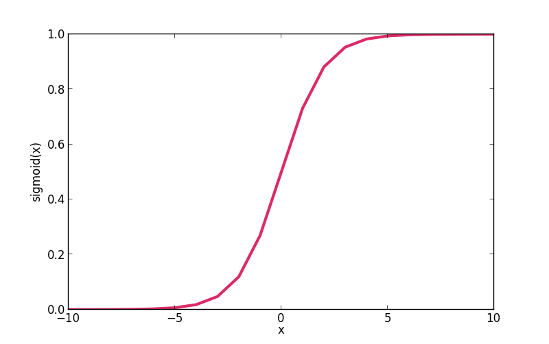
引数として与えたシンボル(スカラー)を冪指数とするネイピア数の冪乗を返す。
x = T.dscalar('x')
exp_x = T.exp(x)
sigmoid_x = 1.0 / (1.0 + T.exp(-x))
f = function([x], [exp_x, sigmoid_x])
for x in [-4, -2, -1, 0, 1, 2, 4]:
    print x, f(x)
# Create Sigmoid Curve
X = range(-10,11)
Y = []
for x in X:
    Y.append(f(x)[1])
import matplotlib.pyplot as plt
plt.plot(X, Y)
plt.show()
-4 [array(0.01831563888873418), array(0.01798620996209156)]
-2 [array(0.1353352832366127), array(0.11920292202211755)]
-1 [array(0.36787944117144233), array(0.2689414213699951)]
0 [array(1.0), array(0.5)]
1 [array(2.718281828459045), array(0.7310585786300049)]
2 [array(7.38905609893065), array(0.8807970779778823)]
4 [array(54.598150033144236), array(0.9820137900379085)]
引数として与えたシンボル(スカラー)の自然対数を返す。tensor.log2() および tensor.log() を用いることで、底を2または10とした対数を返すこともできる。
x = T.dscalar('x')
log_x = T.log(x)
log2_x = T.log2(x)
log10_x = T.log10(x)
f = function([x], [log_x, log2_x, log10_x])
f(8)
[array(2.0794415416798357), array(3.0), array(0.9030899869919435)]
引数として与えた2つのシンボル(ベクトルか行列)の内積を返す。
x1, x2 = T.dvectors('x1', 'x2')
dot_x = T.dot(x1, x2)
f = function([x1, x2], dot_x)
f([1, 2, 3], [6, -5, 4])
array(8.0)
共有変数
theano.shared を用いて共有変数を宣言することができる。共有変数は、複数の関数から参照することができる。値の参照には shared.get_value() を、値の変更には shared.set_value() を用いる。
s = shared(5, name='s')
x = T.iscalar('x')
f1 = function([x], x+s)
f2 = function([x], x-s)
f3 = function([], s*3)
s.get_value()
f1(7), f2(7), f3()
s.set_value(-10)
s.get_value()
f1(7), f2(7), f3()
5
(array(12), array(2), array(15))
-10
(array(-3), array(17), array(-30))
確率モデルのパラメータなどの計算過程で頻繁に更新する変数は、共有変数で宣言しておくことで無駄なメモリコピーを削減できる。theano.function のパラメータの1つである updates と組み合わせることで効率的な計算が可能となる。
state = shared(0)
inc = T.iscalar('inc')
accumulator = function([inc], state, updates=[(state, state+inc)])
decrementor = function([inc], state, updates=[(state, state-inc)])
state.get_value()
accumulator(5)
state.get_value()
decrementor(3)
state.get_value()
0
array(0)
5
array(5)
2
応用例:ロジスティック回帰
上述した基本的な使い方、微分の計算、共有変数を組み合わせることで、ロジスティック回帰を実装することができる (公式チュートリアルより引用)。最急降下法についてはこちらの記事を参照。
import numpy
import theano
import theano.tensor as T
rng = numpy.random

N = 400
feats = 784
D = (rng.randn(N, feats), rng.randint(size=N, low=0, high=2))
training_steps = 10000

# Declare Theano symbolic variables
x = T.matrix("x")
y = T.vector("y")
w = theano.shared(rng.randn(feats), name="w")
b = theano.shared(0., name="b")
print "Initial model:"
print w.get_value(), b.get_value()

# Construct Theano expression graph
p_1 = 1 / (1 + T.exp(-T.dot(x, w) - b))   # Probability that target = 1
prediction = p_1 > 0.5                    # The prediction thresholded
xent = -y * T.log(p_1) - (1-y) * T.log(1-p_1) # Cross-entropy loss function
cost = xent.mean() + 0.01 * (w ** 2).sum()# The cost to minimize
gw, gb = T.grad(cost, [w, b])             # Compute the gradient of the cost
                                          # (we shall return to this in a
                                          # following section of this tutorial)

# Compile
train = theano.function(
          inputs=[x,y],
          outputs=[prediction, xent],
          updates=((w, w - 0.1 * gw), (b, b - 0.1 * gb)))
predict = theano.function(inputs=[x], outputs=prediction)

# Train
for i in range(training_steps):
    pred, err = train(D[0], D[1])

print "Final model:"
print w.get_value(), b.get_value()
print "target values for D:", D[1]
print "prediction on D:", predict(D[0])
コメントを残す